Reading-Notes-for-Advanced-Software-Development-in-Python-Course
Dunder Methods
Dunder or magic methods in Python are the methods having two prefix and suffix underscores in the method name. Dunder here means “Double Under (Underscores)”. These are commonly used for operator overloading.
Let’s look at various “dunder” methods to have the better understanding of various features Python provides.
Object Initialization: init
“__ init__” is a reseved method in python classes. It is known as a constructor in object oriented concepts. This method is called when an object is created from the class and it allow the class to initialize the attributes of a class.
Example:
class Car(object):


    def __init__(self, model, color, company, speed_limit):
        self.color = color
        self.company = company
        self.speed_limit = speed_limit
        self.model = model
Object Representation: str, repr
__str __ This method returns the string representation of the object. This method is called when print() or str() function is invoked on an object.
This method must return the String object. If we don’t implement __str __ () function for a class, then built-in object implementation is used that actually calls __repr __() function.
Python __repr __ function returns the object representation. It could be any valid python expression such as tuple, dictionary, string etc.
This method is called when repr() function is invoked on the object, in that case, __repr __() function must return a String otherwise error will be thrown.
Example:
class Person:

    def __init__(self, personName, personAge):
        self.name = personName
        self.age = personAge

    def __repr__(self):
        return {'name':self.name, 'age':self.age}

    def __str__(self):
        return 'Person(name='+self.name+', age='+str(self.age)+ ')'
Iteration: len, getitem, reversed
The built-in function len() calls the magic method __len __(). len () is the public interface you use to get the length of an object. The __len __ method is the implementation that an object that supports the concept of length is expected to implement. You normally shouldn’t call dunder methods directly, although there are cases where it’s required.
And this is a repeating pattern in Python:
len() and __len__()
iter() and __iter__()
next() and __next__()
format() and __format__()
bool() and __bool__()
hash() and __hash__()
repr() and __repr__()
str() and __str__()
Statistics in Python — Probability
Probability and Statistics are the foundational pillars of Data Science. In fact, the underlying principle of machine learning and artificial intelligence is nothing but statistical mathematics and linear algebra. Often developers will encounter situations, especially in Data Science, where they have to read some research paper which involves a lot of maths in order to understand a particular topic.
A random variable is a variable whose possible values are numerical outcomes of a random phenomenon. There are two types of random variables, discrete and continuous.
A continuous random variable is one which takes an infinite number of possible values. Since the continuous random variable is defined over an interval of values, it is represented by the area under a curve (or the integral).
The probability distribution of a continuous random variable, known as probability distribution functions, are the functions that take on continuous values.
The curve, which represents the probabilty distribution function is often known as a density curve.
-
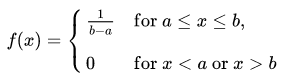
Uniform Distribution
- any interval of numbers of equal width has an equal probability
- the curve describing the distribution is a rectangle, with constant height across the interval and 0 height elsewhere.
-
the area under the curve must be equal to 1
#### In Python
You can visualize uniform distribution in python with the help of a random number generator acting over an interval of numbers (a,b). You need to import the uniform function from scipy.stats module.
from scipy.stats import uniform
n = 10000
start = 10
width = 20
data_uniform = uniform.rvs(size=n, loc = start, scale=width)
The uniform function generates a uniform continuous variable between the specified interval via its loc and scale arguments. This distribution is constant between loc and loc + scale. The size arguments describe the number of random variates.
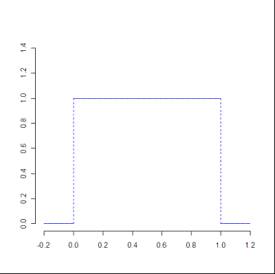
- Normal Distribution
A normal distribution has a bell-shaped density curve described by its mean μ and standard deviation σ. The density curve is symmetrical, centered about its mean, with its spread determined by its standard deviation showing that data near the mean are more frequent in occurrence than data far from the mean.
Below is the figure describing what the distribution looks like:
#### In Python
You can generate a normally distributed random variable using scipy.stats module’s norm.rvs() method. The loc argument corresponds to the mean of the distribution. scale corresponds to standard deviation and size to the number of random variates. If you want to maintain reproducibility, include a random_state argument assigned to a number. You can visualize the distribution just like you did with the uniform distribution, using seaborn’s distplot functions.
    from scipy.stats import norm
    # generate random numbers from N(0,1)
    data_normal = norm.rvs(size=10000,loc=0,scale=1)

    ax = sns.distplot(data_normal,
              bins=100,
              kde=True,
              color='skyblue',
              hist_kws={"linewidth": 15,'alpha':1})
    ax.set(xlabel='Normal Distribution', ylabel='Frequency')
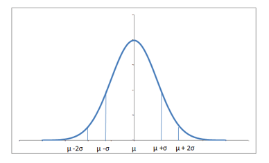
Normal distribution is a particularly important kind of probability distribution. In statistics, it is the values of our data that are being distributed. Here, the x-axis is the values of our data, and the y-axis is the count of each of these values. Here’s the same picture of the normal distribution, but labelled according to a probability and statistical context:
In a probability context, the high point in a normal distribution represents the event with the highest probability of occurring. As you get farther away from this event on either side, the probability drops rapidly, forming that familiar bell-shape.
The high point in a statistical context actually represents the mean. As in probability, as you get farther from the mean, you rapidly drop off in frequency. That is to say, extremely high and low deviations from the mean are present but exceedingly rare.