Reading-Notes-for-Advanced-Software-Development-in-Python-Course
Graphs
A graph is a pictorial representation of a set of objects where some pairs of objects are connected by links. The interconnected objects are represented by points termed as vertices, and the links that connect the vertices are called edges. The various terms and functionalities associated with a graph is described in great detail in our tutorial here. In this chapter we are going to see how to create a graph and add various data elements to it using a python program.
Graphs are networks consisting of nodes connected by edges or arcs. In directed graphs, the connections between nodes have a direction, and are called arcs; in undirected graphs, the connections have no direction and are called edges. We mainly discuss directed graphs. Algorithms in graphs include finding a path between two nodes, finding the shortest path between two nodes, determining cycles in the graph (a cycle is a non-empty path from a node to itself), finding a path that reaches all nodes (the famous “traveling salesman problem”), and so on. Sometimes the nodes or arcs of a graph have weights or costs associated with them, and we are interested in finding the cheapest path.
Graphs are used to represent many real-life applications: Graphs are used to represent networks. The networks may include paths in a city or telephone network or circuit network. Graphs are also used in social networks like linkedIn, Facebook. For example, in Facebook, each person is represented with a vertex(or node). Each node is a structure and contains information like person id, name, gender, and locale. See this for more applications of graph.
Here is some common terminology used when working with Graphs:
- Vertex - A vertex, also called a “node”, is a data object that can have zero or more adjacent vertices.
- Edge - An edge is a connection between two nodes.
- Neighbor - The neighbors of a node are its adjacent nodes, i.e., are connected via an edge.
- Degree - The degree of a vertex is the number of edges connected to that vertex.
Directed and Undirected Graphs
Undirected graphs have edges that do not have a direction. The edges indicate a two-way relationship, in that each edge can be traversed in both directions. This figure shows a simple undirected graph with three nodes and three edges.
The undirected graph we are looking at has 6 vertices and 7 undirected edges.
Vertices/Nodes = {a,b,c,d,e,f}
Edges = {(a,c),(a,d),(b,c),(b,f),(c,e),(d,e),(e,f)}
Directed graphs have edges with direction. The edges indicate a one-way relationship, in that each edge can only be traversed in a single direction. This figure shows a simple directed graph with three nodes and two edges.
The directed graph above has six vertices and eight directed edges
Vertices = {a,b,c,d,e,f}
Edges = {(a,c),(b,c),(b,f),(c,e),(d,a),(d,e)(e,c)(e,f)}
Graph Representation
The following two are the most commonly used representations of a graph.
Adjacency Matrix
Adjacency Matrix is a 2D array of size V x V where V is the number of vertices in a graph. Let the 2D array be adj[][], a slot adj[i][j] = 1 indicates that there is an edge from vertex i to vertex j. Adjacency matrix for undirected graph is always symmetric. Adjacency Matrix is also used to represent weighted graphs. If adj[i][j] = w, then there is an edge from vertex i to vertex j with weight w.

The adjacency matrix for the above example graph is:

Pros: Representation is easier to implement and follow. Removing an edge takes O(1) time. Queries like whether there is an edge from vertex ‘u’ to vertex ‘v’ are efficient and can be done O(1).
Cons: Consumes more space O(V^2). Even if the graph is sparse(contains less number of edges), it consumes the same space. Adding a vertex is O(V^2) time.
Adjacency List
An array of lists is used. The size of the array is equal to the number of vertices. Let the array be an array[]. An entry array[i] represents the list of vertices adjacent to the ith vertex. This representation can also be used to represent a weighted graph. The weights of edges can be represented as lists of pairs. Following is the adjacency list representation of the above graph.

The adjacency matrix for the above example graph is:

Traversals
The traversals itself are like those of trees. Below is a breakdown of how you would traverse a graph.
Breadth First
Breadth First Search (BFS) algorithm traverses a graph in a breadthward motion and uses a queue to remember to get the next vertex to start a search, when a dead end occurs in any iteration.
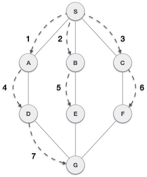
As in the example given above, BFS algorithm traverses from A to B to E to F first then to C and G lastly to D. It employs the following rules.
-
Rule 1 − Visit the adjacent unvisited vertex. Mark it as visited. Display it. Insert it in a queue.
-
Rule 2 − If no adjacent vertex is found, remove the first vertex from the queue.
-
Rule 3 − Repeat Rule 1 and Rule 2 until the queue is empty.
| Step | Traverse | Description |
|---|---|---|
| 1 | 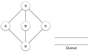 |
Initialize the queue. |
| 2 | 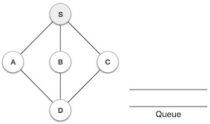 |
We start from visiting S (starting node), and mark it as visited. |
| 3 | 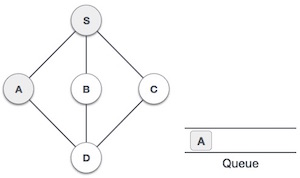 |
We then see an unvisited adjacent node from S. In this example, we have three nodes but alphabetically we choose A, mark it as visited and enqueue it. |
| 4 | 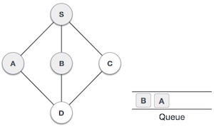 |
Next, the unvisited adjacent node from S is B. We mark it as visited and enqueue it. |
| 5 | 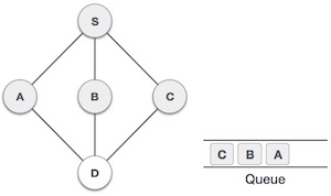 |
Next, the unvisited adjacent node from S is C. We mark it as visited and enqueue it. |
| 6 | 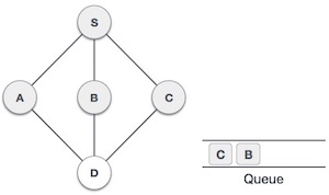 |
Now, S is left with no unvisited adjacent nodes. So, we dequeue and find A. |
| 7 | 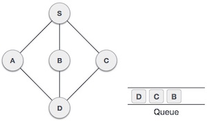 |
From A we have D as unvisited adjacent node. We mark it as visited and enqueue it. |
At this stage, we are left with no unmarked (unvisited) nodes. But as per the algorithm we keep on dequeuing in order to get all unvisited nodes. When the queue gets emptied, the program is over.
Depth First
Depth First Search (DFS) algorithm traverses a graph in a depthward motion and uses a stack to remember to get the next vertex to start a search, when a dead end occurs in any iteration.
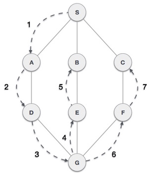
As in the example given above, DFS algorithm traverses from S to A to D to G to E to B first, then to F and lastly to C. It employs the following rules.
-
Rule 1 − Visit the adjacent unvisited vertex. Mark it as visited. Display it. Push it in a stack.
-
Rule 2 − If no adjacent vertex is found, pop up a vertex from the stack. (It will pop up all the vertices from the stack, which do not have adjacent vertices.)
-
Rule 3 − Repeat Rule 1 and Rule 2 until the stack is empty.
| Step | Traverse | Description |
|---|---|---|
| 1 | 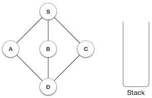 |
Initialize the stack. |
| 2 | 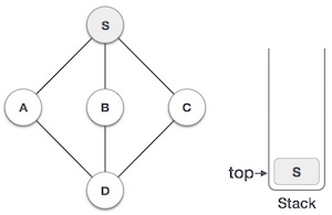 |
Mark S as visited and put it onto the stack. Explore any unvisited adjacent node from S. We have three nodes and we can pick any of them. For this example, we shall take the node in an alphabetical order. |
| 3 | 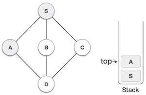 |
Mark A as visited and put it onto the stack. Explore any unvisited adjacent node from A. Both S and D are adjacent to A but we are concerned for unvisited nodes only. |
| 4 | 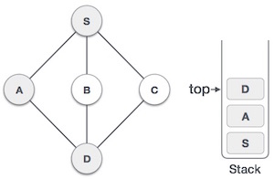 |
Visit D and mark it as visited and put onto the stack. Here, we have B and C nodes, which are adjacent to D and both are unvisited. However, we shall again choose in an alphabetical order. |
| 5 | 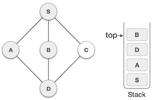 |
We choose B, mark it as visited and put onto the stack. Here B does not have any unvisited adjacent node. So, we pop B from the stack. |
| 6 | 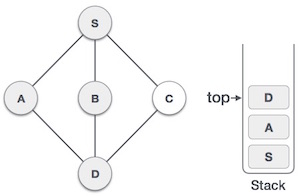 |
We check the stack top for return to the previous node and check if it has any unvisited nodes. Here, we find D to be on the top of the stack. |
| 7 | 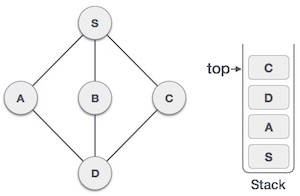 |
Only unvisited adjacent node is from D is C now. So we visit C, mark it as visited and put it onto the stack. |
As C does not have any unvisited adjacent node so we keep popping the stack until we find a node that has an unvisited adjacent node. In this case, there’s none and we keep popping until the stack is empty.
Generate a graph using Dictionary in Python
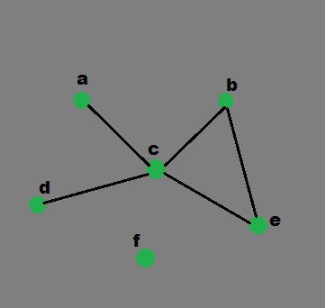
The keys of the dictionary used are the nodes of our graph and the corresponding values are lists with each nodes, which are connecting by an edge. This simple graph has six nodes (a-f) and five arcs:
a -> c
b -> c
b -> e
c -> a
c -> b
c -> d
c -> e
d -> c
e -> c
e -> b
It can be represented by the following Python data structure. This is a dictionary whose keys are the nodes of the graph. For each key, the corresponding value is a list containing the nodes that are connected by a direct arc from this node.
graph = { "a" : ["c"],
          "b" : ["c", "e"],
          "c" : ["a", "b", "d", "e"],
          "d" : ["c"],
          "e" : ["c", "b"],
          "f" : []
        }
Graphical representation of above example:
Remark: Usually, a Python dictionary throws a KeyError if you try to get an item with a key that is not currently in the dictionary. defaultdict allows that if a key is not found in the dictionary, then instead of a KeyError being thrown, a new entry is created. The type of this new entry is given by the argument of defaultdict.
from collections import defaultdict

# function for adding edge to graph
graph = defaultdict(list)
def addEdge(graph,u,v):
    graph[u].append(v)

# definition of function
def generate_edges(graph):
    edges = []

    # for each node in graph
    for node in graph:

        # for each neighbour node of a single node
        for neighbour in graph[node]:

            # if edge exists then append
            edges.append((node, neighbour))
    return edges

# declaration of graph as dictionary
addEdge(graph,'a','c')
addEdge(graph,'b','c')
addEdge(graph,'b','e')
addEdge(graph,'c','d')
addEdge(graph,'c','e')
addEdge(graph,'c','a')
addEdge(graph,'c','b')
addEdge(graph,'e','b')
addEdge(graph,'d','c')
addEdge(graph,'e','c')

# Driver Function call
# to print generated graph
print(generate_edges(graph))
Outpuy:
[('a', 'c'), ('c', 'd'), ('c', 'e'), ('c', 'a'), ('c', 'b'),
('b', 'c'), ('b', 'e'), ('e', 'b'), ('e', 'c'), ('d', 'c')]