Reading-Notes-for-Advanced-Software-Development-in-Python-Course

Pandas

The pandas package is the most important tool in the field of Data Scientists and Analysts working in Python today.

Pandas is a high-level data manipulation tool developed by Wes McKinney. It is built on the Numpy package meaning a lot of the structure of NumPy is used or replicated in Pandas. Data in pandas is often used to feed statistical analysis in SciPy, plotting functions from Matplotlib, and machine learning algorithms in Scikit-learn.

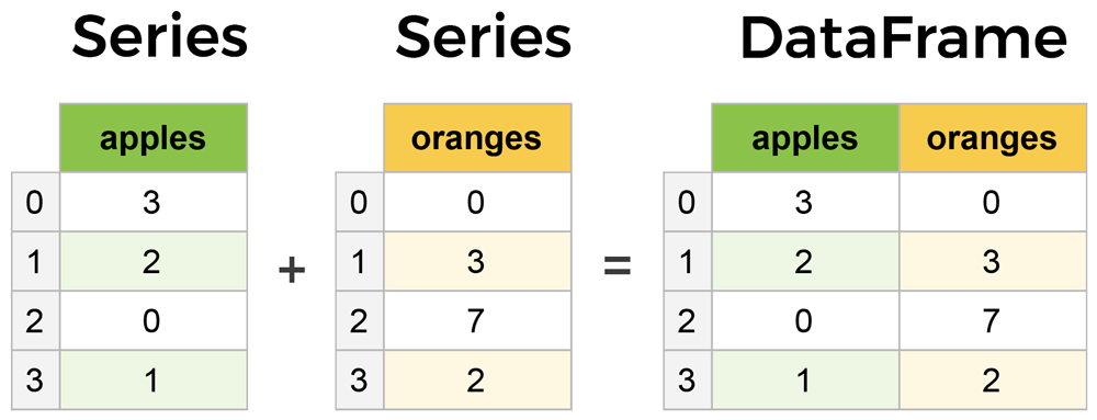
The primary two components of pandas are the Series and DataFrame. A Series is essentially a column, and a DataFrame is a multi-dimensional table made up of a collection of Series.

core

DataFrames and Series are quite similar in that many operations that you can do with one you can do with the other, such as filling in null values and calculating the mean.

Object creation

Creating a Series by passing a list of values, letting pandas create a default integer index:

  In [3]: s = pd.Series([1, 3, 5, np.nan, 6, 8])

  In [4]: s
  Out[4]: 
  0    1.0
  1    3.0
  2    5.0
  3    NaN
  4    6.0
  5    8.0

Creating a DataFrame by passing a NumPy array, with a datetime index and labeled columns:

  In [5]: dates = pd.date_range('20130101', periods=6)

  In [6]: dates
  Out[6]: 
  DatetimeIndex(['2013-01-01', '2013-01-02', '2013-01-03', '2013-01-04',
              '2013-01-05', '2013-01-06'],
              dtype='datetime64[ns]', freq='D')

  In [7]: df = pd.DataFrame(np.random.randn(6, 4), index=dates, columns=list('ABCD'))

  In [8]: df
  Out[8]: 
                  A         B         C         D
  2013-01-01  0.469112 -0.282863 -1.509059 -1.135632
  2013-01-02  1.212112 -0.173215  0.119209 -1.044236
  2013-01-03 -0.861849 -2.104569 -0.494929  1.071804
  2013-01-04  0.721555 -0.706771 -1.039575  0.271860
  2013-01-05 -0.424972  0.567020  0.276232 -1.087401
  2013-01-06 -0.673690  0.113648 -1.478427  0.524988

Viewing data

To view the top and bottom rows of the frame use head and tail.

    In [13]: df.head()
    Out[13]: 
                    A         B         C         D
    2013-01-01  0.469112 -0.282863 -1.509059 -1.135632
    2013-01-02  1.212112 -0.173215  0.119209 -1.044236
    2013-01-03 -0.861849 -2.104569 -0.494929  1.071804
    2013-01-04  0.721555 -0.706771 -1.039575  0.271860
    2013-01-05 -0.424972  0.567020  0.276232 -1.087401

    In [14]: df.tail(3)
    Out[14]: 
                    A         B         C         D
    2013-01-04  0.721555 -0.706771 -1.039575  0.271860
    2013-01-05 -0.424972  0.567020  0.276232 -1.087401
    2013-01-06 -0.673690  0.113648 -1.478427  0.524988

Example:

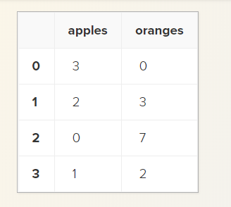
Let’s say we have a fruit stand that sells apples and oranges. We want to have a column for each fruit and a row for each customer purchase. To organize this as a dictionary for pandas we could do something like:

    data = {
        'apples': [3, 2, 0, 1], 
        'oranges': [0, 3, 7, 2]
    }

And then pass it to the pandas DataFrame constructor:

    purchases = pd.DataFrame(data)

    purchases

panda

Each (key, value) item in data corresponds to a column in the resulting DataFrame.

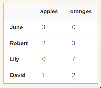
Let’s chnge the index of the dataframe:

    purchases = pd.DataFrame(data, index=['June', 'Robert', 'Lily', 'David'])

    purchases

panda

Now we can locate a customer’s order by using their name:

    purchases.loc['June']

    OUT:
        apples     3
        oranges    0
        Name: June, dtype: int64

To read data from CSV files all you need is a single line to load in the data:

    df = pd.read_csv('students.csv')

CSVs don’t have indexes like our DataFrames, so all we need to do is just designate the index_col when reading:

    df = pd.read_csv('students.csv', index_col=0)

Read and Write to Excel

    pd.read_excel('file.xlsx')
    df.to_excel('dir/myDataFrame.xlsx',  sheet_name='Sheet1')

Selection

Getting

Get one element
```
s['b']
-5
```

Get subset of a DataFrame

df[1:]
Country     Capital   Population
1  India    New Delhi 1303171035
2  Brazil   Brasilia  207847528

Setting

Set index a of Series to a value
```
  s['a'] = 6
```

Sort and Rank

Sort by labels along an axis
```
  df.sort_index()
```
Sort by the values along an axis
```
  df.sort_values(by='Country') 
```
Assign ranks to entries
```
  df.rank()
```

Summary

Sum of values
```
  df.sum()
```
Cumulative sum of values
```
  df.cumsum()
```
Minimum/maximum values
```
  df.min()/df.max()
```
Minimum/Maximum index value
```
  df.idxmin()/df.idxmax() 
```
Summary statistics
```
  df.describe()
```
Mean of values
```
  df.mean()
```